The Fourier Transform is an important tool in Image Processing, and is directly
related to filter theory, since a filter, which is a convolution in the spatial
domain (=the image), is a simple multiplication in the spectral domain (= the FT
of the image)!
Most other tutorials about Fourier Transforms of images are in boring greyscale.
Even, many programs and plugins available that can calculate the FT on images
only support greyscale. In times where 24 and 32 bit color are getting old, we
cannot accept this any longer! This tutorial is in 24-bit
color,
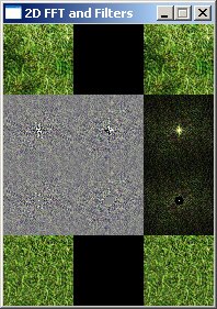
by doing the FT on each colorchannel separately. Here's an example where the FT
of an image is used to make a tillable grass texture look better:
There is also another way to calculate the FT of color images however, by using
quaternions instead of complex numbers, which can convert an image of 4 channels
to another image with 4 channels.
Before beginning with the Fourier Transform on images, which is the 2D version
of the FT, we'll start with the easier 1D FT, which is often used for audio and
electromagnetical signals.
To fully understand this tutorial, it'd be interesting to know about complex
numbers, their magnitude (amplitude), and argument (phase). If you'd like to
learn more about these, there's an appendix about complex numbers (one of the
other html files), or find a tutorial with google.
Signals and Spectra
Before starting with the Fourier Transform, an introduction about Signals and
Spectra is in place. As signals, for now consider signals in the time, like
audio and electromagnetic signals. If you plot such a signal in function of
time, a simple signal could look like this:
This is a sine wave, so if this'd be an audio signal, you'd hear a pure tone
with only 1 frequency (like the beep of a PC speaker, or a very pure flute). The
grey curve behind the red curve represents the amplitude of the signal, which is
always positive.
The spectrum of a signal contains for every frequency, how much of this
frequency is in the signal. Since the signal above is a sine, it has only one
frequency, so the spectrum would be very simple: only one value will be positive
(= the frequency of the sine curve), and all others are zero. So the spectrum
would have a single peak. A spectrum has two sides however: the negative side on
the left, and the positive side on the right. The negative side contains
negative frequencies. For real signals (with no imaginary part), like audio
signals are, the negative side of the spectrum is always a mirrored version of
the positive side. So for the sine signal above, the positive side will have a
single peak, and this peak will be mirrored in the negative side. This is what
it's spectrum looks like:
The white curve represents the amplitude of the signal. The red and green curve
represent the real and imaginary part of the spectrum, respectively, but a
spectrum is raraly represented that way. Normally, both the amplitude and
phase of a spectrum are given, but
since there's not that much interesting info for us in it now, the phase isn't
included.
Let's study another example now: the same sine, but with a DC component added:
sin(x)+C. The name DC component comes from electronics, where it stands for
Direct Current (as opposed to Alternating Current). The DC component in any
signal, is the time average of it. A sine signal has time average 0, but if
however, you add a constant to the sine, the signals time average will become
that constant. This adding of the constant, results in the sine signal being
raised higher above the horizontal axis:
Such a constant, or DC component, has frequency 0. So we can expect that the
spectrum will get an extra peak at the origin, and indeed, it has:
So, if the spectrum of a signal is non-zero at the origin, you know that it's
time average isn't zero and it has a DC component! The further away from the
origin to the left or right a peak is, the higher the frequency it represents,
so a peak far to the right (and left) means that the signal contains a high
frequency component. Note that an audio signal never has a DC component, since
nobody can produce or hear it. Electrical signals can have it however.
Now let's look at a signal which is the sum of two sine functions: the second
sine function has the double frequency of the first, so the curve has the shape
sin(x)+sin(2*x):
Since there are now two sines with two different frequencies, we can expect two
peaks on the positive side of the spectrum (and two more on the negative side
since it's the mirrored version):
If the two sines both have a different phase (i.e. one of the two sines is
shifted horizontally), the amplitude of the spectum will still be the same, only
the phase will be different, but the phase isn't shown here.
Arbitrary sound signals, such as a spoken word, consist of an infinite sum (or
integral) of infinitely much sine functions, all with a different frequency, and
all with their own amplitude and phase, and the spectrum is the perfect plot to
view how much of each frequency is in the signal. Such a spectrum won't just
have a few peaks, but will be a continuous function.
There are a few special functions with a special spectrum:
The Dirac impuls is a signal that is zero everywhere, except at the origin,
where it's infinite. That is the ideal version for continuous functions, for a
discrete function on a computer it can as well be represented as a single peak
with finite height at the origin.
Such a peak sounds like a popping sound in an audio signal, and contains ALL
frequencies. That's why it's spectrum looks like this (the horizontal black
line):
The spectrum is positive everywhere, so every frequency is contained in the
signal. This also means that, to get such a peak as a sum of sine functions, you
have to add infinitely much elementary sine functions all with the same
amplitude, and all shifted with a certain phase, they'll cancel each other out,
except at the origin, hence the peak.
Note that it's possible to intepret the spectrum as a time signal (a constant DC
signal), and that then the red function can be seen as it's spectrum (a peak at
zero, since a DC signal has frequency 0). This duality is one of the interesting
properties of the Fourier Transform as we'll see later.
Finally, another special signal is the sinc(x) function; sinc(x) = sin(x)/x:
It's spectrum is a rectangular pulse (here only an approximation of it because
the spectrum was calculated using only 128 points):
Again because of the duality between a signal and it's spectrum, a rectangular
time signal will have a sinc function as it's spectrum.
Spectra are also used to study the color of light. These are exactly the same
thing, since light too is a 1-dimensional signal containing different
frequencies, some of which the eye happens to be sensitive to. The spectrum
shows for every frequency, how much of it is in the light, just the same as the
audio spectrum does for audio signals.
An MP3 player like Winamp also shows the spectrum of the audio signal it's
playing (but it varies with time because they calculate the spectrum each time
again for the last few milliseconds), and spectra of audio signals can be used
to detect bass, treble and vocals in music, for speach recognition, audio
filters, etc... Since this is a tutorial about computer graphics, I won't go any
deeper in this however.
Often, the spectrum is drawn on a logarithmical scale instead of a linear one
like here, then the amplitude is expressed in decibels (dB).
The Fourier Transform
So how do you calculate the spectrum of a given signal? With the Fourier
Transform!
The Continuous Fourier Transform, for use on continuous signals, is defined as
follows:
And the Inverse Continuous Fourier Transform, which allows you to go from the
spectrum back to the signal, is defined as:
F(w) is the spectrum, where w represents the frequency, and f(x) is the signal
in the time where x represents the time. i is sqrt(-1), see complex number
theory.
Note the similarity between both transforms, which explains the duality between
a signal and it's spectrum.
A computer can't work with continuous signals, only with finite discrete
signals. Those are finite in time, and have only a discrete set of points (i.e.
the signal is sampled). One of the properties of the Fourier Transform and it's
inverse is, that the FT of a discrete signal is periodic. Since for a computer
both the signal and the specrum must be discrete, both the signal and spectrum
will be periodic. But by taking only one period of it, we get our finite signal.
So if you're taking the DFT of a signal or an image on the computer,
mathematicaly speaking, that signal is infinitely repeated, or the image
infinitely tiled, and so is the spectrum. A nice property is that both the
signal and the spectrum will have the same number of discrete points, so the DFT
of an image of 128*128 pixels will also have 128*128 pixels.
Since the signal is finite in time, the infinite borders of the integrals can be
replaced by finite ones, and the integral symbol can be replaced by a sum. So
the DFT is defined as:
And the inverse as:
This looks already much more programmable on a computer, to program the FT, you
have to do the calculation for every n, so you get a double for loop (one for
every n, and one for every k, which is the sum). The exponential of the
imaginary number can be replaced by a cos and a sin by using the famous formuma
e^ix = cosx + isinx. More on programming it follows further in this tutorial.
There are multiple definitions of the DFT, for example you can also do the
division through N in the forward DFT instead of the inverse one, or divide
through sqrt(N) in both. To plot it on a computer, the best result is gotten by
dividing through N in the forward DFT.
Properties of The Fourier Transform
A signal is often denoted with a small letter, and it's fourier transform or
spectrum with a capital letter. The relatoin between a signal and it's spectrum
is often denoted with f(x) <--> F(w),
with the signal on the left and it's spectrum on the right.
The Fourier Transform has some interesting properties, some of which make it
easier to understand why spectra of certain signals have a certain shape.
Don't take this as a proper list however, some scaling factors like 2*pi are
left away, they're not that important and can be left away or depending if you
use frequency or pulsation. Handbooks of Sigal Processing and sites like
Wikipedia and Mathworld contain much more complete and mathematically correct
tables of FT properties. We're most interested in the shape of the functions and
not the scale.
Linearity
f(x)+g(x) <--> F(w)+G(w)
a*f(x) <--> a*F(w)
This means that if you add/substract two signals, their spectra are
added/substracted as wall, and if you increase/decrease the amplitude of the
signal, the amplitude of it's spectrum will be increased/decreased with the same
factor.
Scaling
f(a*x) <--> (1/a) * F(w/a)
This means that if you make the function wider in the x-direction, it's spectrum
will become smaller in the x-direction, and vica versa. The amplitude will also
be changed.
Time Shifting
f(x-x0) <--> (exp(-i*w*x0)) * F(w)
Since the only thing that happens if you shift the time, is a multiplication of
the Fourier Transform with the exponential of an imaginary number, you won't see
the difference of a time shift in the amplitude of the spectrum, only in the
phase.
Frequency Shifting
(exp(-i*w0*x))*f(x)<-->F(w-w0)
This is the dual of the time shifting.
Duality or Symmetry
if f(x) <--> F(w)
then F(x) <--> f(-w)
Apart from some scaling factors at least. Because of this property, for example,
the spectrum of a rectangular pulse is a sinc function and at the same time the
spectrum of a sinc function is a rectangular pulse.
Symmetry Rules
These are only a few of the symmetry rules:
The Fourier Transform of a real even signal is real and even (i.e. it's
symmetrical, mirrored around the y-axis)
The Fourier Transform of a real odd signal is imaginary and odd (odd
means it's assymetrical, mirrored around the origin point)
Since arbitrary real signals are always a sum of an even and an odd
function, the Fourier Transform of a real signal has an even real part and
an odd imaginary part, and the Amplitude is thus always symmetrical.
In the same way, the amplitude of FT's of pure imaginary signals are
symmetrical, but the FT of complex signals isn't always symmetrical.
Convolution Theorem
Convolution is an operation between two functions that is defined as an
integral, but can also be explained as follows:
Take 2 functions, for example two rectangle functions f1(x) and f2(x). Keep one
of the rectangles at a fixed position. Mirror the second one around the y axis
(this doesn't have a lot of effect on a rectangle). Then shift this second
function over a value u, where u goes from -infinity to +infinity.
The resulting function g(u), the convolution of f1(x) and f2(x), takes u as a
parameter. For a certain u, multiply f1 and the shifted and mirrored f2 with
each other, and take area under the result (by integrating it). This area is the
value of g(u) for that u! This has to be done for every u to know the complete
result. For example, for the two rectangle functions, as we start at
u=-infinity, g(u) is 0 because the two rectangles don't overlap, and
multiplication of the two functions will thus result in the zero function, which
has zero area. As u moves to the right, g(u) will remain 0 all the time, until
finally the two rectangles start overlapping. Now the more we go to the right,
the larger the area will become, until it reaches it's maximum, so g(u) is
rising. Then, the rectangles are overlapping less and less again as the second
one moves more to the right, and the value of g(u) decreases again. Finally g(u)
reaches zero again and remains so until +infinity. The resulting g(u) is thus a
triangle function.
This is what filters of painting programs that don't use the FT do in 2D. The
image is then the function that remains at fixed position, while the filter
matrix moves around the whole image, and you calculate the value of every pixel
by multiplying every element of the matrix with every corresponding pixel of the
image the matrix overlaps. For large filter matrices this is a lot of work. You
can create your own filter matrices in painting programs like Paint Shop Pro and
Photoshop by using the "User Defined" filter.
Correlation is almost the same as convolution, except you don't have to mirror
the second function.
The convolution theorem sais that, convolving two functions in the time domain
corresponds to multiplying their spectra in the fourier domain, and vica versa.
This multiplication is a much easier operation than convolution.
Since filters, too, can be described in the time and the fourier domain (called
the impulse response and transfer function of the filter respectively), and
linear filters do a convolutoin in the time domain, in the frequency domain this
corresponds to multiplying the transfer function of the filter with the spectrum
of the signal. The impulse response of the filter in the time domain is the
response of the filter to a dirac impuls (see earlier), and the transfer
function of the filter is the Fourier Transform of the impulse response.
For us, the Convolution Theorem will come in handy when we experiment with the
Fourier Transformations of signals and images.
Programming The 1D Fourier Transform
Here's the code of a simple program that'll calculate the FT of a given signal,
and will plot both the signal and the FT. Put it in the main.cpp file.
First the variables and functions are declared. N will be the number of discrete
points in the signal. For the signal and it's spectrum, respectively a small f
or g and capital F or G are used, as it's also done in mathematics.
		const int N = 128; //yeah ok, we use old fashioned fixed size arrays here

double fRe[N]; //the function's real part, imaginary part, and amplitude
double fIm[N];
double fAmp[N];
double FRe[N]; //the FT's real part, imaginary part and amplitude
double FIm[N];
double FAmp[N];
const double pi = 3.1415926535897932384626433832795;

void DFT(int n, bool inverse, double *gRe, double *gIm, double *GRe, double *GIm);
//Calculates the DFT
void plot(int yPos, double *g, double scale, bool trans, ColorRGB color);
//plots a function
void calculateAmp(int n, double *ga, double *gRe, double *gIm);
//calculates the amplitude of a complex function
The main function creates a sine signal, and will then use the other functions
to calculate the FT and plot it.
int main(int /*argc*/, char */*argv*/[])
{
  screen(640, 480, 0, "1D DFT");
  cls(RGB_White);

  for(int x = 0; x < N; x++)
  {
    fRe[x] = 25 * sin(x / 2.0); //generate a sine signal.  Put anything else you like here.
    fIm[x] = 0;
  }

  //Plot the signal
  calculateAmp(N, fAmp, fRe, fIm);
  plot(100, fAmp, 1.0, 0, ColorRGB(160, 160, 160));
  plot(100, fIm, 1.0, 0, ColorRGB(128, 255, 128));
  plot(100, fRe, 1.0, 0, ColorRGB(255, 0, 0));

  DFT(N, 0, fRe, fIm, FRe, FIm);

  //Plot the FT of the signal
  calculateAmp(N, FAmp, FRe, FIm);
  plot(350, FRe, 12.0, 1, ColorRGB(255, 128, 128));
  plot(350, FIm, 12.0, 1, ColorRGB(128, 255, 128));
  plot(350, FAmp, 12.0, 1, ColorRGB(0, 0, 0));

  drawLine(w / 2, 0, w / 2, h - 1, ColorRGB(128, 128, 255));
  redraw();
  sleep();

  return 0;
}
Then comes the function that does the actual work (albeit with a very suboptimal
algorithm here): the DFT function
void DFT(int n, bool inverse, double *gRe, double *gIm, double *GRe, double *GIm)
{
  for(int w = 0; w < n; w++)
  {
    GRe[w] = GIm[w] = 0;
    for(int x = 0; x < n; x++)
    {
      double a = -2 * pi * w * x / float(n);
      if(inverse) a = -a;
      double ca = cos(a);
      double sa = sin(a);
      GRe[w] += gRe[x] * ca - gIm[x] * sa;
      GIm[w] += gRe[x] * sa + gIm[x] * ca;
    }
    if(!inverse)
    {
      GRe[w] /= n;
      GIm[w] /= n;
    }
  }
}
It takes 4 arrays as parameters: *gRe and *gIm to read from (these are the real
and imaginary part of the signal), and *GRe and *GIm to write the results to
(these are the FT of the signal). Both the input and output are complex numbers,
which is why two arrays (a real and an imaginary one) are needed. n is the size
of the signal (and the arrays), so it's the number of discrete points in the
signal.
The first for loop with w going from 0 to n-1 means that a calculation is needed
for every single point of the result. The second for loop, with x going from 0
to n, means that every point of the input signal needs to be taken in account,
it's the sum from the mathematical definition of the DFT. The exponential
function is changed by the formula e^ix = cosx + isinx, and the real and
imaginary part are calculated seperatly. Afterwards the values are divided
through n, so that the values are reasonably small enough to plot them on the
screen.
By setting "inverse" to true, it can also calculate the IDFT (Inverse Discrete
Fourier Transform), but this isn't used in this example. The only differences
are a different sign in the exponential function and no division through n.
Next, the plot function takes a single array as parameter, and will draw the
signal or spectrum contained in this array on screen with a color you want using
lines and filled circles. You can also use a parameter "shift" to bring the
edges to the center and vica versa. This is useful for a better representation
of the Fourier Transform: normally the result of the DFT has the low frequency
components on the sides, and the highest frequency in the center. Since the
result is in fact periodic, bringing the sides to the center is the same as
moving the plot half a period.
void plot(int yPos, double *g, double scale, bool shift, ColorRGB color)
{
  drawLine(0, yPos, w - 1, yPos, ColorRGB(128, 128, 255));
  for(int x = 1; x < N; x++)
  {
    int x1, x2, y1, y2;
    int x3, x4, y3, y4;
    x1 = (x - 1) * 5;
    //Get first endpoint, use the one half a period away if shift is used
    if(!shift) y1 = -int(scale * g[x - 1]) + yPos;
    else y1 = -int(scale * g[(x - 1 + N / 2) % N]) + yPos;
    x2 = x * 5;
    //Get next endpoint, use the one half a period away if shift is used
    if(!shift) y2 = -int(scale * g[x]) + yPos;
    else y2 = -int(scale * g[(x + N / 2) % N]) + yPos;
    //Clip the line to the screen so we won't be drawing outside the screen
    clipLine(x1, y1, x2, y2, x3, y3, x4, y4);
    drawLine(x3, y3, x4, y4, color);
    //Draw circles to show that our function is made out of discrete points
    drawDisk(x4, y4, 2, color);
  }
}
And finally, the function calculateAmp calculates the amplitude given the real
and imaginary part, so you can plot the amplitude too.
//Calculates the amplitude of *gRe and *gIm and puts the result in *gAmp
void calculateAmp(int n, double *gAmp, double *gRe, double *gIm)
{
  for(int x = 0; x < n; x++)
  {
    gAmp[x] = sqrt(gRe[x] * gRe[x] + gIm[x] * gIm[x]);
  }
}
The output of this program is as follows:
The red function is the input function, which is a sine, and the black funtion
at the bottom is the amplitude of it's spectrum, which is calculated by the DFT
function. The green curves are the imaginary parts.
The Fast Fourier
Transform
The above DFT function correctly calculates the Discrete Fourier Transform, but
uses two for loops of n times, so it takes O(n�) arithmetical operations. A
faster algorithm is the Fast Fourier Transform or FFT, which uses only O(n*logn)
operations. This makes a big difference for very large n: if n would be 1024,
the DFT function would take 1048576 (about 1 million) loops, while the FFT would
use only 10240.
The FFT works by splitting the signal into two halves: one halve contains all
the values with even index, the other all the ones with odd index. Then, it
splits up these two halves again, etc..., recursivily. Due to this, a
requirement is that the size of the signal, n, must be a power of 2. There exist
other FFT versions that can work on signals that can have length n*m where both
n and m are primes, but that goes beyond the scope of this tutorial.
Here's a new version of the DFT function, called FFT, which uses the Fast
Fourier Transform instead. The FFT algorithm used here is called the Radix-2
algorithm, by Cooley-Tukey, developed 1965. You can add it to the previous
program and change the function call of it to FFT to test it out.
First, this function will calculate the logarithm of n, needed for the
algorithm.
void FFT(int n, bool inverse, double *gRe, double *gIm, double *GRe, double *GIm)
{
  //Calculate m=log_2(n)
  int m = 0;
  int p = 1;
  while(p < n)
  {
    p *= 2;
    m++;
  }
Next, Bit Reversal is performed. Because of the way the FFT works, by splitting
the signal in it's even and odd components every time, the algorithm requires
that the input signal is already in the form where all odd components come
first, then the even ones, and so on in each of the halves. This is the same as
reversing the bits of the index of each value (for example the second value,
with index 0001 will now get index 1000 and this go to the center), hence the
name.
      //Bit reversal
  GRe[n - 1] = gRe[n - 1];
  GIm[n - 1] = gIm[n - 1];
  int j = 0;
  for(int i = 0; i < n - 1; i++)
  {
    GRe[i] = gRe[j];
    GIm[i] = gIm[j];
    int k = n / 2;
    while(k <= j)
    {
      j -= k;
      k /= 2;
    }
    j += k;
  }
Next the actual FFT is performed. Mathematically speaking it's a recursive
function, but this is a modified version to work non-recursively, it'd be way
too hard to pass complete arrays to a recursive function every time. ca and sa
still represent the cosine and sine, but are calculated with the half-angle
formulas and initual values -1.0 and 0.0 (cos and sin of pi): each loop, ca and
sa represent the cosine and sine of half the angle as the previous loop.
  //Calculate the FFT
  double ca = -1.0;
  double sa = 0.0;
  int l1 = 1, l2 = 1;
  for(int l = 0; l < m; l++)
  {
    l1 = l2;
    l2 *= 2;
    double u1 = 1.0;
    double u2 = 0.0;
    for(int j = 0; j < l1; j++)
    {
      for(int i = j; i < n; i += l2)
      {
        int i1 = i + l1;
        double t1 = u1 * GRe[i1] - u2 * GIm[i1];
        double t2 = u1 * GIm[i1] + u2 * GRe[i1];
        GRe[i1] = GRe[i] - t1;
        GIm[i1] = GIm[i] - t2;
        GRe[i] += t1;
        GIm[i] += t2;
      }
      double z =  u1 * ca - u2 * sa;
      u2 = u1 * sa + u2 * ca;
      u1 = z;
    }
    sa = sqrt((1.0 - ca) / 2.0);
    if(!inverse) sa =- sa;
    ca = sqrt((1.0 + ca) / 2.0);
  }
Finally, the values are divided through n if it isn't the inverse DFT.
      //Divide through n if it isn't the IDFT
  if(!inverse)
  for(int i = 0; i < n; i++)
  {
    GRe[i] /= n;
    GIm[i] /= n;
  }
}
The function reads from *gRe and *gIm again and stores the result in *GRe and
*GIm.
There are 3 nested loops now in the FFT part, but only the first one goes from 0
to n-1, the other two together only loop log_2(n) times. For this small signal
of only 128 values you probably won't notice any increase in speed because both
DFT and FFT are calculated instantly (unless you're working on some computer
from the '40s), but on bigger signals, on 2D signals, and in applications where
the FT has be be calculated over and over in real time, it'll make an important
difference.
Filters
In the Fourier Domain, it's easy to apply some filters. All you have to do is
multiply the spectrum with the transfer function of the filter.
Low pass filters only let through components with low frequencies (for example
the bass from music), while High Pass filters let only components with high
frequencies through. You can also make Band Pass and Band Stop filters, which
let through or block components with a certain frequency. Amplifiers multiply
the whole spectrum with a constant value, and you can of course make filters
that amplify certain frequencies, or triangular filters that weaken higher
frequencies more and more, etc...
So to make for example a Low Pass filter, multiply the spectrum with a
rectangular function with the rectangle around the origin. All the low frequency
components will then be kept, while the high ones are multiplied by zero and are
thus filtered away.
Here's a part of code for a program that'll first allow you to select different
signals and watch their FT, and after pressing the space key, will allow you to
choose different filters on the spectrum, and it'll calculate the inverse FT to
see how the original signal is affected by the filter.
First all variables and functions are declared.
		const int N = 128; //yeah ok, we use old fashioned fixed size arrays here

double fRe[N]; //the function's real part, imaginary part, and amplitude
double fIm[N];
double fAmp[N];
double FRe[N]; //the FT's real part, imaginary part and amplitude
double FIm[N];
double FAmp[N];
const double pi = 3.1415926535897932384626433832795;

void FFT(int n, bool inverse, double *gRe, double *gIm, double *GRe, double *GIm); //Calculates the DFT
void plot(int yPos, double *g, double scale, bool trans, ColorRGB color); //plots a function
void calculateAmp(int n, double *ga, double *gRe, double *gIm); //calculates the amplitude of a
complex function
The main function starts here. It enters the first loop, this loop will allow
you to choose a function. The parameters p1 and p2 can be changed to modify the
amplitude and/or width of some of the functions.
int main(int /*argc*/, char */*argv*/[])
{
  screen(640, 480, 0, "Fourier Transform and Filters");
  for(int x = 0; x < N; x++) fRe[x] = fIm[x] = 0;
  bool endloop = 0, changed = 1;
  int n = N;
  double p1 = 25.0, p2 = 2.0;
  while(!endloop)
  {
    if(done()) end();
    readKeys();
This is inside the loop after it has read the keys. Every key has another action
assiciated to it to create a certain function, for example if you press the g
key (SDLK_g) it'll put a sum of two sines in fRe[x]. The arrow keys also have
some actions to set the imaginary part to 0, equal to the real part, or a
modified version of the real part. Finally, the space keys sets "endloop" to
true so that the first loop will end.
Not all keys are included here, because it's very messy and big code. Only a few
are shown as an example, the rest is in the downloadable source file.
		if(keyPressed(SDLK_a)) {for(int x = 0; x < n; x++) fRe[x] = 0; changed = 1;} //zero
    if(keyPressed(SDLK_b)) {for(int x = 0; x < n; x++) fRe[x] = p1; changed = 1;} //constant
    if(keyPressed(SDLK_c)) {for(int x = 0; x < n; x++) fRe[x] = p1 * sin(x / p2); changed = 1;} //sine


    //ETCETERA... *snip*

    if(keyPressed(SDLK_SPACE)) endloop = 1;
This is the last part of the first loop, where it draws the chosen function,
calculates it's FT, and draws that one too.
After the first loop has ended, the second part of the main function starts.
First, an extra spectrum buffer is created, so that both the original spectrum
and it's filtered version can be remembered. Then the second loop starts.
  //The original FRe2, FIm2 and FAmp2 will become multiplied by the filter
  double FRe2[N];
  double FIm2[N];
  double FAmp2[N];
  for(int x = 0; x < N; x++)
  {
    FRe2[x] = FRe[x];
    FIm2[x] = FIm[x];
  }
  cls();
  changed = 1; endloop = 0;
  while(!endloop)
  {
    if(done()) end();
    readKeys();
Now the keys all change the spectrum in a certain way: they'll aplly a filter.
Low Pass filters (LP) set the spectrum to 0, except around the origin. High Pass
filters (HP) do the oposite.
Not all keys are shown here, because it's very messy and big code. Only a few
are shown as an example, the rest is in the downloadable source file in a more
closely packed form.
Again, if a key was pressed, the new spectrum is drawn, and the inverse FFT is
performed to draw the filtered version of the original function. If you press
escape the program will end.
The functions FFT, plot and calculateAmp are identical to the ones explained
earlier and aren't included here anymore.
There's not much new in this code, the functions FFT, plot and calculateAmp are
still the same, but by playing with this program you can see the effects of Low
Pass (LP), High Pass (HP) and a few other filters. Just follow the instructions
on screen.
For example, here, a signal which is the sum of 5 sines and a DC component
(gotten by pressing the "p" key) is shown together with it's spectrum, and then,
respectively, a LP and a HP are applied to it:
The original signal:
An LP Filter:
A HP Filter
Here, the same is done with a step function (gotten by pressing the "e" key):
An LP filter on it:
A HP filter on it. This filter filters out almost only the DC component, so two
almost-flat lines remain in the signal: