The extension of the Fourier Transform to 2D is actually pretty simple. First
you take the 1D FT of every row of the image, and then on this result you take
the 1D FT of every column.
Here follows the code of a program that does exactly that, and two alternative
functions that do the same are given in it: one will use the 2D version of the
slow DFT, and the other the 2D version of the Fast Fourier Transform (FFT). The
program will first calculate the FT of the image, and then calculate the Inverse
FT of the result, to check if the formula is working correctly: if it gives back
the original it works. You can freely change between calls to DFT2D()
and FFT2D() in the main function, and you'll notice that the
DFT2D() function is very slow now, while the FFT2D() function
works very fast.
Because an RGB image has 3 color channels, the FT is calculated for each color
channel separately, so in fact 3 greyscale FT's are calculated.
The program requires that there's a 24-bit color, 128*128 bitmap image
pics/test.png (path relative to the program).
First again all the variables and functions are declared.
N and M are the width and height of the image in pixels.
The arrays for the signal and it's spectrum are now 3-dimensional: 2 dimensions
for the size, and 1 dimension for the RGB color components. The class ColorRGB
can't be used here because more precision is required for FT, that's why the
color components are put in a double array instead; index 0 represents red,
index 1 green, and index 2 is blue.
There are two versions of the FT functions here, the slow DFT2D and the fast
FFT2D.
//yeah, we're working with fixed sizes again...
const int N = 128; //the width of the image
const int M = 128; //the height of the image

double fRe[N][M][3], fIm[N][M][3], fAmp[N][M][3]; //the signal's real part, imaginary part,
and amplitude
double FRe[N][M][3], FIm[N][M][3], FAmp[N][M][3]; //the FT's real part, imaginary part
and amplitude
double fRe2[N][M][3], fIm2[N][M][3], fAmp2[N][M][3]; //will become the signal again after
IDFT of the spectrum
double FRe2[N][M][3], FIm2[N][M][3], FAmp2[N][M][3]; //filtered spectrum

double pi = 3.1415926535897932384626433832795;

void draw(int xpos, int yPos, int n, int m, double *g, bool shift, bool neg128);
void DFT2D(int n, int m, bool inverse, double *gRe, double *gIm, double *GRe, double *GIm);
void calculateAmp(int n, int m, double *ga, double *gRe, double *gIm);
The main function first loads an image, and then sets the signal to that image.
Next, it draws the image. It draws the real part, the imaginary part (which is
0!), and the amplitude, which looks the same as the real part.
Then it calculates the FT of the image, by using the DFT2D function, but you can
as well change this to FFT2D instead: it'll go faster then. Then it draws the
just calculated spectrum.
Finally, it calculates the inverse FT of that spectrum again and draws the
result, this is only to check if the functions are working correctly: if you get
the original image back, they are.
		int main(int /*argc*/, char */*argv*/[])
{
  screen(N * 3, M * 3, 0, "2D DFT and FFT");

  std::vector<ColorRGB> img;
  unsigned long dummyw, dummyh;
  if(loadImage(img, dummyw, dummyh, "pics/test.png"))
  {
    print("image pics/test.png not found");
    redraw();
    sleep();
    cls();
  }

  //set signal to the image
  for(int x = 0; x < N; x++)
  for(int y = 0; y < M; y++)
  {
    fRe[x][y][0] = img[N * y + x].r;
    fRe[x][y][1] = img[N * y + x].g;
    fRe[x][y][2] = img[N * y + x].b;
  }

  //draw the image (real, imaginary and amplitude)
  calculateAmp(N, M, fAmp[0][0], fRe[0][0], fIm[0][0]);
  draw(0, 0, N, M, fRe[0][0], 0, 0);
  draw(N, 0, N, M, fIm[0][0], 0, 0);
  draw(2 * N, 0, N, M, fAmp[0][0], 0, 0);

  //calculate and draw the FT of the image
  DFT2D(N, M, 0, fRe[0][0], fIm[0][0], FRe[0][0], FIm[0][0]); //Feel free to
  change this to FFT2D
  calculateAmp(N, M, FAmp[0][0], FRe[0][0], FIm[0][0]);
  draw(0, M, N, M, FRe[0][0], 1, 1);
  draw(N, M, N, M, FIm[0][0], 1, 1);
  draw(2 * N, M, N, M, FAmp[0][0], 1, 0);

  //calculate and draw the image again
  DFT2D(N, M, 1, FRe[0][0], FIm[0][0], fRe2[0][0], fIm2[0][0]); //Feel free to
  change this to FFT2D
  calculateAmp(N, M, fAmp2[0][0], fRe2[0][0], fIm2[0][0]);
  draw(0, 2 * M, N, M, fRe2[0][0], 0, 0);
  draw(N, 2 * M, N, M, fIm2[0][0], 0, 0);
  draw(2 * N, 2 * M, N, M, fAmp2[0][0], 0, 0);

  redraw();
  sleep();
  return 0;
}
This is the DFT2D function, it's really just the same as the 1D versions of DFT
which was explained in an earlier section, only with an extra loop to do the
calculation for every row or column, and repeated twice (for the columns, and
for the rows), and this separately for every color component. The function take
now two parameters for the dimensions: m and n, because an image is 2D. The
parameter inverse can be set to true to do the inverse calculations instead.
Again *gRe and *gIm are the input arrays, and *GRe and *GIm the output arrays.
In this 2D version, the values are divided through m for the normal DFT and
through n for the inverse DFT. There are also definitions where you should
divide through m*n in one direction and through 1 in the other, or though
sqrt(m*n) in both, but it doesn't really matter which one you pick, as long as
the forward FT and the inverse together give the original image back. The
version here gives the nicest results to draw.
void DFT2D(int n, int m, bool inverse, double *gRe, double *gIm, double *GRe, double *GIm)
{
  std::vector<double> Gr2(m * n * 3);
  std::vector<double> Gi2(m * n * 3); //temporary buffers

  //calculate the fourier transform of the columns
  for(int x = 0; x < n; x++)
  for(int c = 0; c < 3; c++)
  {
    print(" % done",8, 0, RGB_White, 1);
    print(50 * x / n, 0, 0, RGB_White, 1);
    if(done()) end();
    redraw();
    //This is the 1D DFT:
    for(int w = 0; w < m; w++)
    {
      Gr2[m * 3 * x + 3 * w + c] = Gi2[m * 3 * x + 3 * w + c] = 0;
      for(int y = 0; y < m; y++)
      {
        double a= 2 * pi * w * y / float(m);
        if(!inverse)a = -a;
        double ca = cos(a);
        double sa = sin(a);
        Gr2[m * 3 * x + 3 * w + c] += gRe[m * 3 * x + 3 * y + c] * ca -
		gIm[m * 3 * x + 3 * y + c] * sa;
        Gi2[m * 3 * x + 3 * w + c] += gRe[m * 3 * x + 3 * y + c] * sa +
		gIm[m * 3 * x + 3 * y + c] * ca;
      }

    }
  }
  //calculate the fourier transform of the rows
  for(int y = 0; y < m; y++)
  for(int c = 0; c < 3; c++)
  {
    print(" % done",8, 0, RGB_White, 1);
    print(50 + 50 * y / m, 0, 0, RGB_White, 1);
    if(done()) end();
    redraw();
    //This is the 1D DFT:
    for(int w = 0; w < n; w++)
    {
      GRe[m * 3 * w + 3 * y + c] = GIm[m * 3 * w + 3 * y + c] = 0;
      for(int x = 0; x < n; x++)
      {
        double a = 2 * pi * w * x / float(n);
        if(!inverse)a = -a;
        double ca = cos(a);
        double sa = sin(a);
        GRe[m * 3 * w + 3 * y + c] += Gr2[m * 3 * x + 3 * y + c] * ca -
		Gi2[m * 3 * x + 3 * y + c] * sa;
        GIm[m * 3 * w + 3 * y + c] += Gr2[m * 3 * x + 3 * y + c] * sa +
		Gi2[m * 3 * x + 3 * y + c] * ca;
      }
      if(inverse)
      {
        GRe[m * 3 * w + 3 * y + c] /= n;
        GIm[m * 3 * w + 3 * y + c] /= n;
      }
      else
      {
        GRe[m * 3 * w + 3 * y + c] /= m;
        GIm[m * 3 * w + 3 * y + c] /= m;
      }
    }
  }
}
And here's the Fast Fourier Transform again, in 2D this time. The same can be
said about this function as for the DFT2D function. The explanation of the FFT
was already done in an earlier section.
void FFT2D(int n, int m, bool inverse, double *gRe, double *gIm, double *GRe, double *GIm)
{
  int l2n = 0, p = 1; //l2n will become log_2(n)
  while(p < n) {p *= 2; l2n++;}
  int l2m = 0; p = 1; //l2m will become log_2(m)
  while(p < m) {p *= 2; l2m++;}

  m = 1 << l2m; n = 1 << l2n; //Make sure m and n will be powers of 2, otherwise you'll
  get in an infinite loop

  //Erase all history of this array
  for(int x = 0; x < m; x++) //for each column
  for(int y = 0; y < m; y++) //for each row
  for(int c = 0; c < 3; c++) //for each color component
  {
    GRe[3 * m * x + 3 * y + c] = gRe[3 * m * x + 3 * y + c];
    GIm[3 * m * x + 3 * y + c] = gIm[3 * m * x + 3 * y + c];
  }

  //Bit reversal of each row
  int j;
  for(int y = 0; y < m; y++) //for each row
  for(int c = 0; c < 3; c++) //for each color component
  {
    j = 0;
    for(int i = 0; i < n - 1; i++)
    {
      GRe[3 * m * i + 3 * y + c] = gRe[3 * m * j + 3 * y + c];
      GIm[3 * m * i + 3 * y + c] = gIm[3 * m * j + 3 * y + c];
      int k = n / 2;
      while (k <= j) {j -= k; k/= 2;}
      j += k;
    }
  }
  //Bit reversal of each column
  double tx = 0, ty = 0;
  for(int x = 0; x < n; x++) //for each column
  for(int c = 0; c < 3; c++) //for each color component
  {
    j = 0;
    for(int i = 0; i < m - 1; i++)
    {
      if(i < j)
      {
        tx = GRe[3 * m * x + 3 * i + c];
        ty = GIm[3 * m * x + 3 * i + c];
        GRe[3 * m * x + 3 * i + c] = GRe[3 * m * x + 3 * j + c];
        GIm[3 * m * x + 3 * i + c] = GIm[3 * m * x + 3 * j + c];
        GRe[3 * m * x + 3 * j + c] = tx;
        GIm[3 * m * x + 3 * j + c] = ty;
      }
      int k = m / 2;
      while (k <= j) {j -= k; k/= 2;}
      j += k;
    }
  }

  //Calculate the FFT of the columns
  for(int x = 0; x < n; x++) //for each column
  for(int c = 0; c < 3; c++) //for each color component
  {
    //This is the 1D FFT:
    double ca = -1.0;
    double sa = 0.0;
    int l1 = 1, l2 = 1;
    for(int l=0;l < l2n;l++)
    {
      l1 = l2;
      l2 *= 2;
      double u1 = 1.0;
      double u2 = 0.0;
      for(int j = 0; j < l1; j++)
      {
        for(int i = j; i < n; i += l2)
        {
          int i1 = i + l1;
          double t1 = u1 * GRe[3 * m * x + 3 * i1 + c] - u2 * GIm[3 * m * x + 3 * i1 + c];
          double t2 = u1 * GIm[3 * m * x + 3 * i1 + c] + u2 * GRe[3 * m * x + 3 * i1 + c];
          GRe[3 * m * x + 3 * i1 + c] = GRe[3 * m * x + 3 * i + c] - t1;
          GIm[3 * m * x + 3 * i1 + c] = GIm[3 * m * x + 3 * i + c] - t2;
          GRe[3 * m * x + 3 * i + c] += t1;
          GIm[3 * m * x + 3 * i + c] += t2;
        }
        double z =  u1 * ca - u2 * sa;
        u2 = u1 * sa + u2 * ca;
        u1 = z;
      }
      sa = sqrt((1.0 - ca) / 2.0);
      if(!inverse) sa = -sa;
      ca = sqrt((1.0 + ca) / 2.0);
    }
  }
  //Calculate the FFT of the rows
  for(int y = 0; y < m; y++) //for each row
  for(int c = 0; c < 3; c++) //for each color component
  {
    //This is the 1D FFT:
    double ca = -1.0;
    double sa = 0.0;
    int l1= 1, l2 = 1;
    for(int l = 0; l < l2m; l++)
    {
      l1 = l2;
      l2 *= 2;
      double u1 = 1.0;
      double u2 = 0.0;
      for(int j = 0; j < l1; j++)
      {
        for(int i = j; i < n; i += l2)
        {
          int i1 = i + l1;
          double t1 = u1 * GRe[3 * m * i1 + 3 * y + c] - u2 * GIm[3 * m * i1 + 3 * y + c];
          double t2 = u1 * GIm[3 * m * i1 + 3 * y + c] + u2 * GRe[3 * m * i1 + 3 * y + c];
          GRe[3 * m * i1 + 3 * y + c] = GRe[3 * m * i + 3 * y + c] - t1;
          GIm[3 * m * i1 + 3 * y + c] = GIm[3 * m * i + 3 * y + c] - t2;
          GRe[3 * m * i + 3 * y + c] += t1;
          GIm[3 * m * i + 3 * y + c] += t2;
        }
        double z =  u1 * ca - u2 * sa;
        u2 = u1 * sa + u2 * ca;
        u1 = z;
      }
      sa = sqrt((1.0 - ca) / 2.0);
      if(!inverse) sa = -sa;
      ca = sqrt((1.0 + ca) / 2.0);
    }
  }

  int d;
  if(inverse) d = n; else d = m;
  for(int x = 0; x < n; x++) for(int y = 0; y < m; y++) for(int c = 0; c < 3; c++) //for every value
  of the buffers
  {
    GRe[3 * m * x + 3 * y + c] /= d;
    GIm[3 * m * x + 3 * y + c] /= d;
  }
}
The draw function does what the plot function did in the 1D version: show the
signal on screen. Now this function will draw the signal or spectrum arrays you
feed it as a 24-bit RGB image with the upper left corner at xpos,yPos. The shift
parameter can be used to bring the corners to the center and the center to the
corners, useful for FT's to bring the DC component to the center. The neg128
parameter can be used to draw images that can have negative pixel values: now
gray (RGB color 128, 128, 128) is used as 0, darker colors are negative, and
brighter ones are positive.
		//Draws an image
void draw(int xPos, int yPos, int n, int m, double *g, bool shift, bool neg128) //g is the
image to be drawn
{
  for(int x = 0; x < n; x++)
  for(int y = 0; y < m; y++)
  {
    int x2 = x, y2 = y;
    if(shift) {x2 = (x + n / 2) % n; y2 = (y + m / 2) % m;} //Shift corners to center
    ColorRGB color;
    //calculate color values out of the floating point buffer
    color.r = int(g[3 * m * x2 + 3 * y2 + 0]);
    color.g = int(g[3 * m * x2 + 3 * y2 + 1]);
    color.b = int(g[3 * m * x2 + 3 * y2 + 2]);

    if(neg128) color = color + RGB_Gray;
    //negative colors give confusing effects so set them to 0
    if(color.r < 0) color.r = 0;
    if(color.g < 0) color.g = 0;
    if(color.b < 0) color.b = 0;
    //set color components higher than 255 to 255
    if(color.r > 255) color.r = 255;
    if(color.g > 255) color.g = 255;
    if(color.b > 255) color.b = 255;
    //plot the pixel
    pset(x + xPos, y + yPos, color);
  }
}
The calculateAmp function is also again the same as the 1D version, only with an
extra loop for the 2nd dimension, and another one for the color components. This
function is used to generate the amplitudes of the signals and spectra so that
you can draw those.
//Calculates the amplitude of *gRe and *gIm and puts the result in *gAmp
void calculateAmp(int n, int m, double *gAmp, double *gRe, double *gIm)
{
  for(int x = 0; x < n; x++)
  for(int y = 0; y < m; y++)
  for(int c = 0; c < 3; c++)
  {
    gAmp[m * 3 * x + 3 * y + c] = sqrt(gRe[m * 3 * x + 3 * y + c] *
	gRe[m * 3 * x + 3 * y + c] + gIm[m * 3 * x + 3 * y + c] * gIm[m * 3 * x + 3 * y + c]);
  }
}
Note that, because of the way C++ works, the arrays are passed to the functions
in a special way, and inside the functions they have to be treated as
1-dimensional.
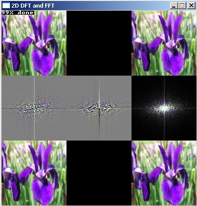
The output of the program is as follows:
On the top row are the real part, imaginary part and amplitude of the image. The
imaginary part of the image is 0.
On the center row are the real part, imaginary part and amplitude of the
spectrum from the image. The real and imaginary part can have negative values,
so they have the "neg128" option enabled to draw them and grey represents 0.
Since the amplitude is always positive, black is 0 there.
The bottom row is again the image, calculated by using the Inverse DFT of the
spectrum. It looks almost the same as the original, a few pixels might slightly
differ in color due to rounding errors.
The text "99% done" only appears if you use the DFT2D function, since it's so
slow (30 seconds on an Athlon 1700+ processor for an 128x128 image) a progress
counter is handy. The FFT2D does the same calculation immediatly, so such a
counter isn't needed.
If you study the spectra of the images, you'll see horizontal and vertical lines
through the center. They're caused by the sides of the image: since
mathematically speaking, the FT is calculated of the image tiled infinite times,
there's an abrupt change when going from one side of the image to the other,
causing the lines in the spectrum.
Some remarks:
If you'd calculate the forward FT instead of the inverse FT to go back
from the spectrum to the image, you get the image upside down.
Both the real and imaginary part of the spectrum are needed to
reconstruct the image out of it, even though the image itself has no
imaginary part.
The FT functions also work on images that have an imaginary part, for
example if a color image would have only 2 color channels, one color channel
could be used as real part and the other as imaginary part.
Even though the image itself is in 24-bit color, which means that each
pixel has 8 bit per color channel, or 256 discrete color values per channel,
the FT of it requires much more precision: both the real and imaginary
component require floating point numbers that can go from -infinity to
+infinity. Otherwise you'll lose information and the image you get back
after doing the inverse FT on it again will look very crappy. The spectra
displayed on the computer screen don't contain all information, since
they're converted back to integers with 256 discrete values.
By taking the DFT of the amplitude of the spectrum of an image, you will
NOT get the original image back at all, since it requires a high precision
real and an imaginary part of the spectrum, not the amplitude.
The
Spectra of Images
You can replace test.png by any 24-bit 128*128 color bitmap you want. You can
even use another size, but then you'll have to change the parameters N and M in
the code (on top). Note that the FFT2D function only works on images with a size
that is a power of two (64x64, 128x256, 256x256... all work), otherwise you'll
have to use the slower DFT2D function.
The spectrum of an image isn't immediatly the most interesting thing (applying
filters on it and then taking the inverse FT again is much more interesting),
but you can still learn a bit about an image by looking at it's spectrum: here
are a few examples, each picture shows the real part of the image, and the
amplitude of the spectrum. To see the real and imaginary part of the spectrum,
run the images through the program yourself.
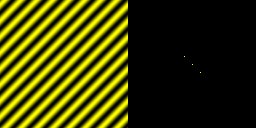
This image is a sine function with a DC component added (because images can only
have positive pixel values): the color of each pixel is 128 + 128 *
sin(pi*y/16.0). If you remember the spectra of 1D signals, you'll remember that
a sine function gave a peak on the negative and positive side, and that the DC
component gave a peak at zero. Here you can see the same in the spectrum: the
center dot is the DC component, and the two others represent the frequency of
the sine function, the one dot is just a mirrored version of the other one.
There are no pixels in the x-direction, because the image is the same everywhere
in that direction.
Here a sine function with a higher frequency is used to generate the image, so
the two dots are further away from the origin to represent the higher frequency.
Remember the scale property of the Fourier Transform? Here it's illustrated very
well: the image contracts, and it's spectrum becomes wider.
In the next image, the sine function doesn't tile: if you'd put the same image
twice on top of each other, you wouldn't see a sine anymore in the y-direction
(while in the previous two examples you would). This isn't considered a real
sine anymore by the spectrum either, and it doesn't contain just two dots, but a
line.
One of the properties of the 2D FT is that if you rotate the image, the spectrum
will rotate in the same direction:
The following image shows the sum of 2 sine functions, each in another direction
(Plasma effects are often made this way):
The following image shows how lines in an image often generate perpendicular
lines in the spectrum:
The sloped lines in the spectrum here are obviously due to the sharp transition
from the sky to the mountain.
The FT of a rectangular function is a 2D sinc function:
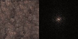
And here's the FT of a tillable texture, since it's tillable there are no abrupt
changes on the horizontal and vertical sides, so there are no horizontal and
vertical lines in the spectrum:
2D Filters
Now comes the most interesting application of the FT on images: you can easily
apply all sorts of filters to the spectrum, again by multiplying them with a 2D
transfer function, or by making some parts of the spectrum zero, or just
applying some whacko formula to the spectrum. After doing that, take the inverse
FT of the modified spectrum to get the filtered image.
Here's part of the code for a program that'll allow you to select different
images (a bitmap, modified versions of it, and some generated functions), and
then after pressing space, allows you to apply different filters and see their
effect.
This code doesn't contain much new, it's much more interesting to run it and
study the results of the filters.
Once again, first come all the declarations of functions and variables. f2 and
F2 will become the buffers for the filtered versions of the original image and
spectrum.
		//yeah, we're working with fixed sizes again...
const int N = 128; //the width of the image
const int M = 128; //the height of the image

double fRe[N][M][3], fIm[N][M][3], fAmp[N][M][3]; //the signal's real part, imaginary part,
and amplitude
double FRe[N][M][3], FIm[N][M][3], FAmp[N][M][3]; //the FT's real part,
imaginary part and amplitude
double fRe2[N][M][3], fIm2[N][M][3], fAmp2[N][M][3]; //will become the signal again
after IDFT of the spectrum
double FRe2[N][M][3], FIm2[N][M][3], FAmp2[N][M][3]; //filtered spectrum

double pi = 3.1415926535897932384626433832795;

void draw(int xpos, int yPos, int n, int m, double *g, bool shift, bool neg128);
void FFT2D(int n, int m, bool inverse, double *gRe, double *gIm, double *GRe, double *GIm);
void calculateAmp(int n, int m, double *ga, double *gRe, double *gIm);
The main function loads a PNG image first, and will then start the first loop,
the loop that lets you try out different modified versions of the PNG image and
some other generated signals:
int main(int /*argc*/, char */*argv*/[])
{
  screen(3 * N,4 * M + 8, 0,"2D FFT and Filters");
  std::vector img;
  unsigned long dummyw, dummyh;
  if(loadImage(img, dummyw, dummyh, "pics/test.png"))
  {
    print("image pics/test.png not found");
    redraw();
    sleep();
    cls();
  }
  //set signal to the image
  for(int x = 0; x < N; x++)
  for(int y = 0; y < M; y++)
  {
    fRe[x][y][0] = img[N * y + x].r;
    fRe[x][y][1] = img[N * y + x].g;
    fRe[x][y][2] = img[N * y + x].b;
  }

  int ytrans=8; //translate everything a bit down to put the text on top

  //set new FT buffers
  for(int x = 0; x < N; x++)
  for(int y = 0; y < M; y++)
  for(int c = 0; c < 3; c++)
  {
    FRe2[x][y][c] = FRe[x][y][c];
    FIm2[x][y][c] = FIm[x][y][c];
  }

  bool changed = 1, endloop = 0;
  while(!endloop)
  {
    if(done()) end();
    readKeys();
Here's a small part of the input part of the first loop, it looks pretty messy
here, only a few keys are shown here, the code for all keys is included in the
downloadable file.
    if(keyPressed(SDLK_a) || changed)
    {
      for(int x = 0; x < N; x++)
      for(int y = 0; y < M; y++)
      for(int c = 0; c < 3; c++)
      {
        fRe2[x][y][c] = fRe[x][y][c];
      } changed = 1;
    } //no effect
    if(keyPressed(SDLK_b))
    {
      for(int x = 0; x < N; x++)
      for(int y = 0; y < M; y++)
      for(int c = 0; c < 3; c++)
      {
        fRe2[x][y][c] = 255 - fRe[x][y][c];
      }
    changed = 1;} //negative
    if(keyPressed(SDLK_c))
    {
      for(int x = 0; x < N; x++)
      for(int y = 0; y < M; y++)
      for(int c = 0; c < 3; c++)
      {
        fRe2[x][y][c] = fRe[x][y][c]/2;
      }
      changed = 1;
    } //half amplitude


    //ETCETERA... *snip*

    if(keyPressed(SDLK_SPACE)) endloop = 1;
If a key was pressed, the new version of the image and it's spectrum will be
drawn. If the first loop was done (by pressing space), the second loop is
initialized:
    if(changed)
    {
      //Draw the image and it's FT
      calculateAmp(N, M, fAmp2[0][0], fRe2[0][0], fIm2[0][0]);
      draw(0, ytrans, N, M, fRe2[0][0], 0, 0);  draw(N, 0+ytrans, N, M,
	  fIm2[0][0], 0, 0);
	  draw(2 * N, 0+ytrans, N, M, fAmp2[0][0], 0, 0); //draw real,
	  imag and amplitude
      FFT2D(N, M, 0, fRe2[0][0], fIm2[0][0], FRe[0][0], FIm[0][0]);
      calculateAmp(N, M, FAmp[0][0], FRe[0][0], FIm[0][0]);
      draw(0,M + ytrans, N, M, FRe[0][0], 1, 1);  draw(N, M + ytrans, N, M,
	  FIm[0][0], 1, 1);
	  draw(2 * N, M + ytrans, N, M, FAmp[0][0], 1, 0); //draw real, imag and amplitude
      print("Press a-z for effects and space to accept", 0, 0, RGB_White,
	  1, ColorRGB(128, 0, 0));
      redraw();
    }
    changed = 0;
  }
  changed = 1;
  while(!done())
  {
    readKeys();
Here's a small part of the input code to apply filters: a Low Pass, High Pass
and Band Pass filter are given. The rest of the keys is in the downloadable
file.
    if(keyPressed(SDLK_f))
    {
      for(int x = 0; x < N; x++)
      for(int y = 0; y < M; y++)
      for(int c = 0; c < 3; c++)
      {
        if(x * x + y * y < 64 || (N - x) * (N - x) + (M - y) * (M - y) < 64 ||
		x * x + (M - y) * (M - y) < 64 || (N - x) * (N - x) + y * y < 64)
        {
          FRe2[x][y][c] = FRe[x][y][c];
          FIm2[x][y][c] = FIm[x][y][c];
        }
        else
        {
          FRe2[x][y][c] = 0;
          FIm2[x][y][c] = 0;
        }
      }
      changed = 1;
    } //LP filter

    if(keyPressed(SDLK_i))
    {
      for(int x = 0; x < N; x++)
      for(int y = 0; y < M; y++)
      for(int c = 0; c < 3; c++)
      {
        if(x * x + y * y > 16 && (N - x) * (N - x) + (M - y) * (M - y)
		> 16 && x * x + (M - y) * (M - y) > 16 && (N - x) *
			(N - x) + y * y > 16)
        {
          FRe2[x][y][c] = FRe[x][y][c];
          FIm2[x][y][c] = FIm[x][y][c];
        }
        else
        {
          FRe2[x][y][c] = 0;
          FIm2[x][y][c] = 0;
        }
      }
      changed = 1;
    } //HP filter

    if(keyPressed(SDLK_s))
    {
      for(int x = 0; x < N; x++)
      for(int y = 0; y < M; y++)
      for(int c = 0; c < 3; c++)
      {
        if((x * x + y * y < 256 || (N - x) * (N - x) + (M - y) * (M - y) < 256 ||
		x * x + (M - y) * (M - y) < 256 || (N - x) * (N - x) + y * y < 256) &&
		(x * x + y * y > 128 && (N - x) * (N - x) + (M - y) * (M - y) > 128 &&
		x * x + (M - y) * (M - y) > 128 && (N - x) * (N - x) + y * y > 128))
        {
          FRe2[x][y][c] = FRe[x][y][c];
          FIm2[x][y][c] = FIm[x][y][c];
        }
        else
        {
          FRe2[x][y][c] = 0;
          FIm2[x][y][c] = 0;
        }
      }
      changed = 1;
    } //BP filter

    //ETCETERA... *snip*
This is the part of the second loop that draws the filtered spectrum and signal,
and the final part of the main function:
if(changed)
{
//after pressing a key: calculate the inverse!
FFT2D(N, M, 1, FRe2[0][0], FIm2[0][0], fRe[0][0], fIm[0][0]);
calculateAmp(N, M, fAmp[0][0], fRe[0][0], fIm[0][0]);
draw(0, 3 * M + ytrans, N, M, fRe[0][0], 0, 0); draw(N, 3 * M + ytrans, N, M, fIm[0][0], 0, 0);
draw(2 * N, 3 * M + ytrans, N, M, fAmp[0][0], 0, 0);
calculateAmp(N, M, FAmp2[0][0], FRe2[0][0], FIm2[0][0]);
draw(0, 2 * M + ytrans, N, M, FRe2[0][0], 1, 1); draw(N, 2 * M + ytrans, N, M, FIm2[0][0], 1, 1);
draw(2 * N, 2 * M + ytrans, N, M, FAmp2[0][0], 1, 0);
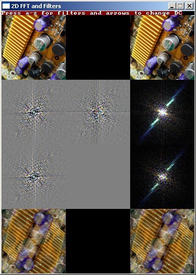
print("Press a-z for filters and arrows to change DC", 0, 0, RGB_White, 1, ColorRGB(128, 0, 0));
redraw();
}
changed=0;
}
return 0;
}
The functions FFT2D, draw and calculateAmp are the same as before again and not
shown here. They're also in the downloadable file.
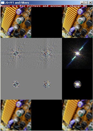
Here's a possible output of the program:
The top row shows the original image, below that is it's spectrum (the amplitude
on the right), the third row shows the spectrum with a low pass filter applied
to it: only the low frequency components remain. The bottom row shows the result
of the Inverse FT on the new spectrum: all high frequency components of the
image are removed, and the image becomes blurred.
Here's another example, which shows what happens if you set the imaginary part
of the spectrum to 0. To get this, first press space and then press the b key in
the program.
More on different types of filters follows in the next sections.