The Excel Formatting Toolbar
A D V E R T I S E M E N T
Excel formatting toolbar normally located near to the top of your screen
as shown here. The toolbar icons have a specific purpose that can change the
outlook of your spreadsheet when you apply formatting to it.

The formatting toolbar icons and functions:Font � to select fonts
from a drop-down list.
Font Size � to select a font size from a drop-down list.
Bold � to apply bold to a selected range.
Italic � to apply italic to a selected range.
Underline � to underline a selected range.
Align Left � to align a selected range to the left.
Center � to center a selected range
Align Right � to align a selected range to the right.
Merge and Center � to merge cells and center text across a selected
range.
Currency Style � to apply currency style to a selected range.
Percent Style � to apply percentage style to a selected range.
Comma Style � to apply comma style to a selected range.
Increase Decimal � to decrease the number of decimal points displayed
in a selected range.
Decrease Decimal � to increase the number of decimal points displayed
in a selected range.
Decrease Indent � to decrease the level of indentation in a selected
range.
Increase Indent � to increase the level of indentation in a selected
range.
Borders � to select and apply borders to a selected range.
Fill Color � to select and apply color to a selected range.
Font Color � to select and apply color to text in a selected range.
The Excel Formatting - FontsTo change the font used in a
cell or range of cells
Select the cell or range of cells you wish to change.
On the Excel Formatting toolbar choose a font from the Font
drop down list.
To change other font characteristics
Select the cell or range you wish to change.
From the Format menu, click Cells.
From the Format Cells dialog box displayed, select the Font tab to
change the Font, font style, or size.
Select the Underline: drop down list box to select a style of
underline or None to remove the underlining.
Select the Color: drop down list box to choose a font color.
In the Effects section, you can tick Strikethrough, Superscript,
or Subscript.
To change all the settings in the dialog box back to the Normal style which
is set in the Style dialog box, tick the Normal font check box.
Select OK to close the Format Cells dialog box.
The Excel Formatting - AlignmentTo align data between the
left and right sides of a cell
Select the cell, or cells, you wish to align.
On the Excel Formatting toolbar, click on the Align Left icon
to align data with the left edge of the cell.
Click on the Align Right icon to align data with the right edge of
the cell.
Click on the Center icon to center data in the cell.
To align data between the top and bottom of a cell
Select the cell, or cells, you wish to align.
From the Format menu, click Cells.
From the Format Cells dialog box displayed, click on the Alignment
tab.
In the Text alignment section, choose the Top, Center, or Bottom
option in the Vertical area to align the data in the cell.
To make the lines of data fit evenly within the height of a cell, tick the
Justify distributed option and click on OK.
To change the orientation of data cells
Select the cell, or cells, you wish to change.
From the Format menu, click Cells.
From the Format Cells dialog box displayed, click on the Alignment
tab.
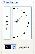
In the Orientation section, you can change the Degrees of the
text or use the mouse to drag the 'red small diamond' up or down. When
satisfied, click on OK.

To wrap multiple lines of data in a cell
Type the data you require into the cell and press Enter. The entry
will appear as one long line and select the cell, or cells, you wish to format.
From the Format menu, click Cells.
From the Format Cells dialog box displayed, click on the Alignment
tab.
In the Text control section, tick the Wrap text check box and
click on OK.
To shrink the text into one cell
Type the data you require into the cell and press Enter.
From the Format menu, click Cells.
From the Format Cells dialog box displayed, click on the Alignment
tab.
In the Text control section, tick the Shrink to fit check box
and click on OK.
To merge several cells
Select the cells that you wish to merge to become one cell.
Right-click on the selected cells, click Format Cells.
From the Format Cells dialog box displayed, click on the Alignment
tab.
In the Text control section, tick the Merge cells check box
and click on OK.
Note: You also can use the Merge and Center icon on the Excel
Formatting toolbar.
The Excel Formatting - ColorsTo change the color of text
Select the cells containing the data you want to change the color.
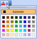
On the Excel Formatting toolbar, click the down arrow next to the
Font Color icon.

Choose a color from the Font Color palette.
The color you selected from the Font Color palette will be displayed
on the new icon face. Click on the icon face to apply the new color to the cell.
To apply colors to cell(s)
Select the cell or range of cells you wish to color.
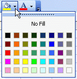
On the Excel Formatting toolbar, click the down arrow next to the
Fill Color icon.
Choose a color from the Fill Color palette.

To turn off the cell(s) color
Select the cell or range of cells you wish to color.
On the Excel Formatting toolbar, click the down arrow next to the
Fill Color icon.
Choose No fill.
The Excel Formatting - NumbersTo change number formatting
using the formatting icons
You can quickly change the formatting of a cell or selected range by using
the following icons on the Formatting toolbar.

| Currency |
12345 will become $12,345.00
|
| Percent |
.25 will become 25%
|
| Comma |
98765 will become 98,765.00
|
| Increase Decimal |
12,345.00 will become 12,345.000
|
| Decrease Decimal |
98,765.00 will become 98,765.0
|
To format a number as a currency
Select the cell or range of cells you want to format.
From the Format menu, click Cells.
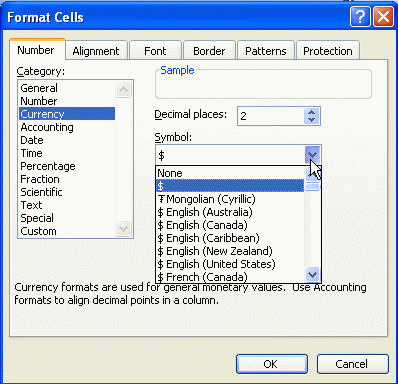
From the Format Cells dialog box displayed, select the Number
tab.
In the Category: section, select Currency.

Select the number of decimal places you require by using the Decimal
places: spin box arrows.
In the Symbol: section drop down list, select the type of currency.
Click OK.
To format a number as a percentage
Select the cell or range of cells you wish to format.
From the Format menu, click Cells.
From the Format Cells dialog box displayed, select the Number
tab.
In the Category: section, select Percentage.
Select the number of decimal places you require by using the Decimal
places: spin box arrows.
Click OK.
|
