Using The Excel Conditional Formatting
A D V E R T I S E M E N T
Excel conditional formatting allows you to apply different formatting
options, such as color, to a cell or cells based on the data in the cell(s).
Here are the 2 easy steps to implement the conditional formatting:
1. Create a set of conditions that control formatting changes in the target
cells.
2. Enter your data. If the conditions you set are met by the data, then the
formatting is applied.
Note: Up to three conditions can be set for a cell, so it is possible to
vary the formatting as the contents of a cell changes.
To format cells using conditional formatting
If we enter the data as illustrated, we can then apply conditional
formatting to it.

Select the range of cells which you wish to apply conditional formatting. In
this example the range would be A1:C5.
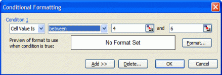
From the Format menu, click Conditional Formatting.

Lets say we wish to highlight all values between 4 and 6, then we would enter
the numbers in the correct fields, as illustrated above.
If we click on the OK button, then no special formatting would be
applied to these values, so next we need to click on the Format button
within this dialog box.

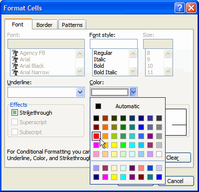
From the normal Format Cells dialog box is displayed, from which we
can specify how data that meets the specified criteria will be displayed.
Select a color for the conditional formatting; choose red, for this example.
When finished click on the OK button to close this dialog box, which
will return to the Conditional Formatting dialog box.
To add the other conditional formats, click the Add button.
Otherwise, click on OK button to close this dialog box.
|
